SLAM & Localization
An MBot in a maze it has never seen. It maps as it drives, picks frontiers to explore, and escapes through a wall that is removed partway through the run. SLAM Toolbox for the map, A* over an obstacle distance grid for the path, a small state machine sequencing the whole thing.
1.0 Summary
The ROB 330 Escape Challenge drops a robot into a maze it has never seen. It has to explore the maze, build a map while it goes, drive back to where it started, and then escape through a wall that gets removed partway through the run.
This is a writeup of how mine worked, on the MBot platform. The map is an obstacle distance grid (Section 3.1), planning is A* over that grid with 8-way expansion (Section 4.0), exploration picks frontiers between known and unknown space (Section 5.0), and a small state machine sequences the whole thing (Section 6.1). It runs in C++ on ROS2, with SLAM Toolbox and lidar for mapping and AprilTags for localization.
2.0 Background & Problem
Autonomous exploration is three problems stacked on each other. The robot needs a representation of what it has seen, a way to plan a path through that representation, and a policy for deciding where to go next. Each one depends on the one before it, so a bad map makes good planning impossible no matter how good the planner is.
2.1 The Challenge
A run has four phases:
- Start in an unknown maze and explore it.
- Build a map while exploring.
- Return to the starting position.
- A wall is removed. Find the opening and escape.
The last phase is the interesting one, because the map the robot spent the whole run building is now wrong in exactly one place, and it has no direct way of being told where.
2.2 Why the Map Comes First
A planner that treats the robot as a point will happily route it through a gap narrower than the robot is. There are two ways to fix that: give the planner a footprint to reason about, or make the map account for the footprint so the planner can stay simple. This took the second option, which is what Section 3.1 is about.
3.0 Map Representation
3.1 Obstacle Distance Grid
A raw occupancy grid says which cells are occupied. That is not enough to plan on safely, so it gets turned into an obstacle distance grid, where every free cell also stores how far it is from the nearest occupied cell. Planning then has a notion of how much clearance a route has, not just whether it fits.
- The environment is assumed to be mostly static while mapping.
- Obstacles are grown to account for the robot's footprint, so the planner can keep modeling the robot as a point.
- Expansion is 8-way, so diagonal travel is allowed and paths do not have to staircase around corners.
3.2 Safety Parameters
Two mechanisms, one hard and one soft:
| Parameter | Value | Effect |
|---|---|---|
| Hard block | 0.05 m | Cells within this distance of an occupied cell are treated as blocked. |
| Safety weight | 0.6 | Biases the path away from obstacles without forbidding those cells. |
The hard block is what keeps the robot from clipping walls. The soft weight is what keeps it off them when there is room to spare, so it drives down the middle of a corridor instead of along one side.
4.0 Planning
4.1 A* on an 8-Connected Grid
Planning is A* over the obstacle distance grid with 8-connected expansion. Diagonal moves cost more than straight ones, and the safety weight from Section 3.2 folds into the cost, so a path that hugs a wall comes out more expensive than one with clearance.
4.2 Heuristic Choice
Euclidean distance pairs naturally with 8-way expansion, since it admits diagonal shortest paths without overestimating them. Two alternatives were considered:
- Manhattan distance, which suits 4-way expansion and overestimates on a grid that allows diagonals.
- Diagonal distance, which is the tighter fit for 8-way movement but was not needed to get good paths here.
Rotation cost is not modeled. It could be, by weighting turn magnitude
into g(x), which would make the planner prefer straighter
routes. On a differential drive robot every turn costs real time, so the
shortest path and the fastest path are not always the same one.
Worth being upfront about: some scripted test cases can fail even when the real runs succeed. Sensor noise and continuous replanning mean the robot does not follow the exact path a fixed test expects.
5.0 Exploration
5.1 Frontier Detection
A frontier is the boundary between space the robot knows is free and space it has not seen yet. A cell is a frontier cell if it is free and adjacent to unknown space.
- Find every frontier cell in the current map.
- Grow and cluster them into connected components, so a whole stretch of frontier cells becomes one frontier instead of hundreds.
- Pick one and drive toward its middle, which maximizes how much new area gets mapped on the way.
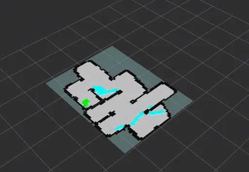
The limitation is noise. Small sensor errors create tiny fake frontiers that are not worth visiting. A gain-based method would score each frontier by how much information gain it is likely to produce and prioritize on that instead of treating them all as targets.
5.2 Centroid Navigation
Driving to a frontier's centroid is simple and it mostly works, but it has three failure modes worth naming:
- The centroid can be unreachable, or sit inside geometry too tight for the robot to fit into.
- It does not prioritize the closest reachable frontier point, so the robot can spend time and battery crossing the map for no reason.
- It treats every frontier as equally worth visiting instead of picking the most promising region.
6.0 Escape
6.1 State Machine
The behavior is sequenced by a small state machine, kept from Lab 12 because it was already clear and reliable:
Initializing → Exploring → Returning Home → Escape
- Initializing. Come up and start mapping.
- Exploring. Repeatedly pick a frontier and drive to it until there are none left.
- Returning Home. Plan a path back to the start.
- Escape. Once the wall is gone, re-explore and drive for the opening.
6.2 Detecting Edge Removal
When the wall comes out, the map is stale. The approach here was to reset the map and let exploration rebuild it, which the challenge allows. With a fresh map the removed wall shows up as a new frontier, and the robot drives for the largest and farthest one first, on the assumption that the exit is the biggest opening.
A full reset throws away a whole run of good mapping to fix one wrong cell, which is the main thing worth improving here.
7.0 Reflection & Next Steps
| Next | Why |
|---|---|
| Tune the safety distance | Cut down wall clips without making narrow corridors unplannable. |
| Phase out stale map values | Detect wall removal by decaying old occupancy instead of resetting everything. |
| Gain-based frontier choice | Score frontiers by expected information gain instead of treating them equally. |
| Rotation cost in the planner | Weight turn magnitude into g(x) so paths prefer fewer turns. |